
안녕하세요 pulluper 입니다.
오늘은 CVPR2017 에 best paper 를 받은 "Densely Connected Convolutional Networks" 에 대해서 알아보고
이해를 위한 간단한 layer 를 pytorch 로 구현 해보겠습니다. :)
1. background
이 시기의 네트워크 들은 점점 깊어지고 (e.g. vgg) 정확해지며, 짧은 connection (short path) 들을 (e.g. resnet)많이 사용하기 시작했습니다. 연결이 있다면 더 학습하기 쉽다고 논문에서 언급합니다.
이러한 observation 들을 가지고 많이 연결을 하여 각 layer 간의 최대한의 정보흐름을 이용하자는 것이 densenet 입니다.
2. Idea
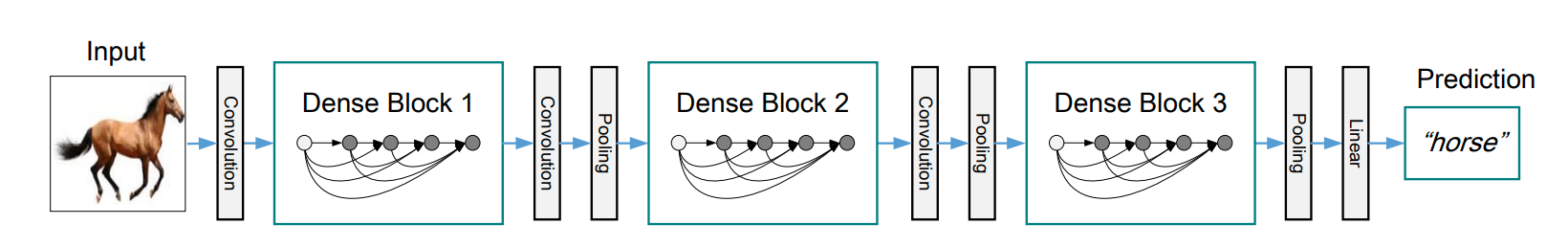
이제 Densenet 의 핵심 아이디어 입니다.
"feed forward 시 각 layer 들이 다른 모든 layer 들과 연결을 합니다!"
위의 사진을 보면, input 을 제외한 4개의 layer 가 있는데, layer 들이 모두 연결되어 있습니다.
논문에서는 이렇게 하면 얻는 다음과 같은 4가지의 장점을 주장합니다.
- vanishing-gradient 문제를 완화 할 수 있다.
- feature propagation을 강화 할 수 있다.
- feature 의 재사용을 할 수 있다.
- parameter 의 수를 줄일 수 있다.
많은 연결을 하였기 때문에 윗쪽의 3가지의 장점은 이해가 조금 가는것 같습니다.
그러나, parameter 의 수는 오히려 늘것 같은데, 왜 줄어드는지 잠시 후 알아보겠습니다.
3. Connections
그렇다면 Densenet 이 실제로 어떻게 연결이 되어있는지 알아보겠습니다.
Densenet 연결을 Resnet과의 비교를 통해서 보면 아래 그림과 같습니다.
왼쪽은 Resnet 의 연결로 feature 들을 그냥 더해줍니다. (channel 축으로)
오른쪽은 Densenet 의 연결로 feature 들을 concatenation 을 통해서 연결해 줍니다. (역시 channel 축으로)
이렇게 되면 어떤 차이가 발생하게 될까요???
둘다 basic block 이라고 가정했을때, resnet 은 output, Input feature channel 이 같다는 것이고,
densenet은 output feature의 channel이 더 커진다는 것 입니다.
이를 위해서 densenet은 한 layer 의 output의 channel 크기를 제한하였는데요. 이를 "Growth rate" 라고 합니다.
이것을 포함해 구현을 위한 논문에서의 설명을 분석해 보겠습니다.
4. Terminology
이번에는 구현을 위해 논문에서 사용하는 용어와 그것이 의미하는 바를 알아보겠습니다!
Growth rate
앞에서 densenet 의 connection을 알아보았는데, concat 을 하기위해서 각 layer 에서의 output 이 똑같은 channel 수로 만들어주는게 좋습니다. 이 output 의 channel 수를 Growth rate 라고 합니다. 이는 hyper parameter 로 Imagenet training 을 위한 Growth rate = 32 입니다.
참고로 densenet의 parameter 를 줄이는 역할을 하는데, output 의 channel을 작게(12, 32..)줄이기 때문에 output 을 만드는 conv 의 weight 를 줄이게 됩니다.
Composite function
pytorch code 로는 다음과 같이 표현될 수 있습니다.
nn.Sequential(nn.BatchNorm2d(input),
              nn.ReLU(inplace=True),
              nn.Conv2d(input, output, 3, padding=1, bias=False))
Bottleneck layers
Darknet 이나 Resnet, Inception 등에서 사용된 bottleneck 이라는 개념은 1x1 convolution으로 channel 을 줄여주고,
이후에 보통 학습을 위한 3x3 convolution 을 이용해서 weight 를 줄이는 구조로 이해하시면 되는데요, 여기서는 다음과 같은 구조를 이용합니다.
BN-ReLU-Conv(1x1)-BN-ReLU-Conv(3x3)
이 구조는 위에서 설명한 bn 이 먼저 나오는 composite function 이 적용되었다고 보시면 되겠습니다.
코드로는 다음과 같이 볼 수 있겠네요
nn.Sequential(nn.BatchNorm2d(64),
              nn.ReLU(inplace=True),
              nn.Conv2d(64, 128, 1, bias=False),

              nn.BatchNorm2d(128),
              nn.ReLU(inplace=True),
              nn.Conv2d(128, 32, 3, padding=1, bias=False),)
pooling layer (Transition layers)
Densenet의 block 은 Composite function으로 이루어진 Bottleneck layer로 이루어집니다. 그런데 여기서는 feature 의 width 와 height 는 줄이지 않습니다. 따라서 block 이 끝난후에 pooling layer 를 사용해서 feature 의 weight 를 줄여줍니다. 그 구조는 다음과 같습니다.
BN(ReLU)-Conv(1x1)-AvgPool(2x2)
nn.Sequential(nn.BatchNorm2d(256),
              nn.ReLU(inplace=True),
              nn.Conv2d(256, 128, 1, bias=False),
              nn.AvgPool2d(kernel_size=2, stride=2)
              )
Compression
Compression은 pooling layer(Transition layer)의 1x1 Convolution layer 에서 channel 을 줄여주는 비율을 말합니다. 위 코드에서 0.5 가 적용된것을 볼 수 있습니다. (256 -> 128)
5. architecture
이 chapter 에서는 dense conectivity 에 대하여 알아보고 첫번째 Dense Block 을 구현 해 보도록 하겠습니다.
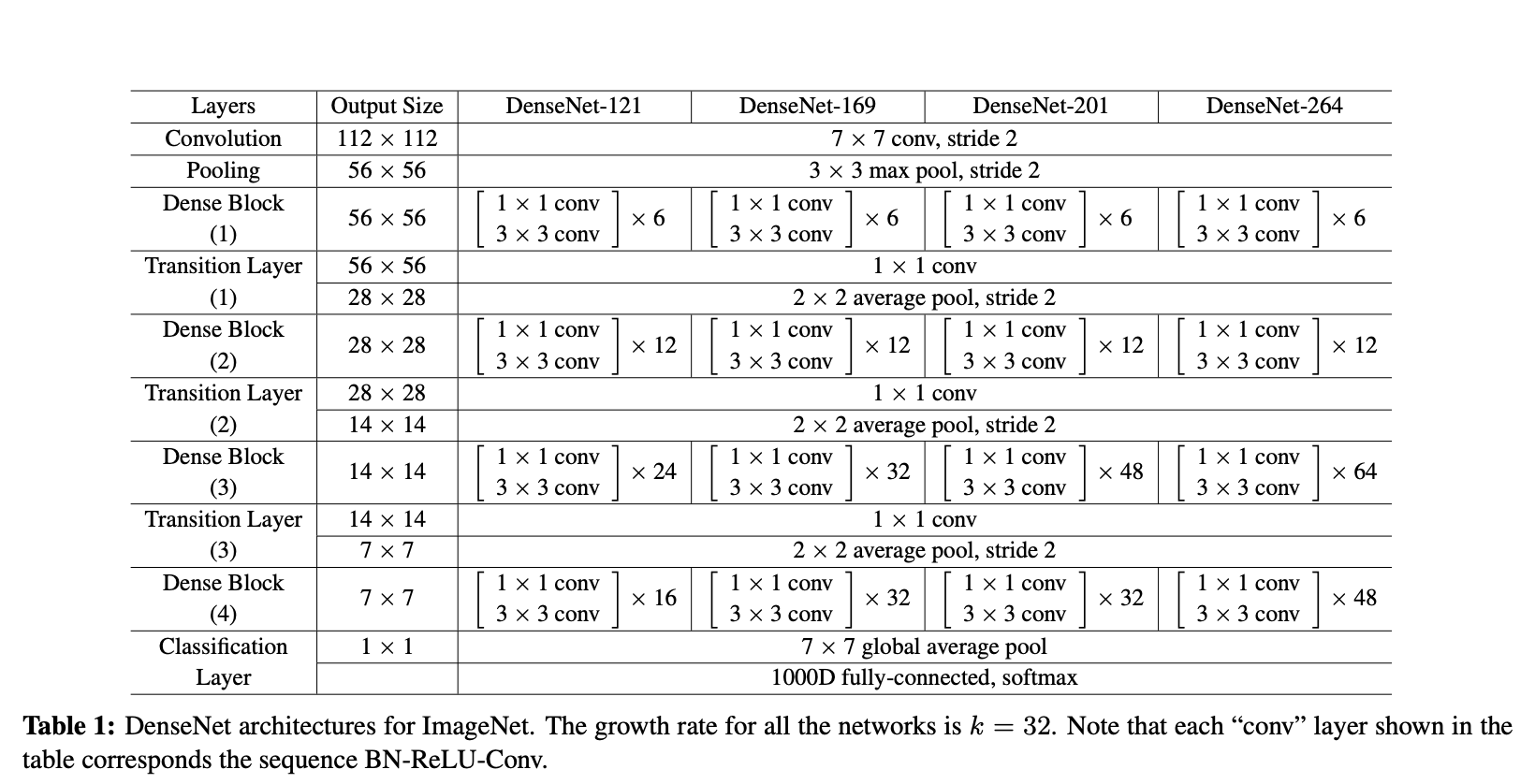
위에서 보는것과 같이 DenseNet-121의 Dense Block (1) 에서 [1 x 1 conv - 3 x 3 conv] 의 bottle neck 구조가 6번 반복되어 있는 것을 볼 수 있습니다. 그런데, Denseblock 내의 어떤 layer 는 그 이전의 layer 들의 output 들의 모든 concat 을 input 으로 받아야 합니다.
그림과 같이 DenseBlock 1 의 layer 는 인풋이 계속 달라집니다.
다음 코드를 보면 DenseBlock 을 이루는 layer 의 input 이 계속 논문에서 말한것 처럼
이후 forward 에서는 layer 를 지날때 마다 concat 을 하여 다음 layer 를 통과시킬 수 있습니다.
이 코드는 이해를 위해 만들어진 코드입니다.
이렇게 하나하나 짜게되면 거의 몇백줄이 소요되겠네요. ㅎㅎ
import torch
import torch.nn as nn
class DenseNet(nn.Module):
def __init__(self, num_classes=1000):
super().__init__()
self.num_classes = num_classes
self.growth_rate = 32
self.base_feature = nn.Sequential(nn.Conv2d(3, 64, 7, stride=2, padding=3, bias=False),
nn.BatchNorm2d(64),
nn.ReLU(inplace=True),
nn.MaxPool2d(kernel_size=3, stride=2, padding=1)
)
self.dense_layer1 = nn.Sequential(nn.BatchNorm2d(64),
nn.ReLU(inplace=True),
nn.Conv2d(64, self.growth_rate * 4, 1, bias=False),
nn.BatchNorm2d(self.growth_rate * 4),
nn.ReLU(inplace=True),
nn.Conv2d(self.growth_rate * 4, self.growth_rate, 3, padding=1, bias=False),
)
self.dense_layer2 = nn.Sequential(nn.BatchNorm2d(96),
nn.ReLU(inplace=True),
nn.Conv2d(96, 128, 1, bias=False),
nn.BatchNorm2d(128),
nn.ReLU(inplace=True),
nn.Conv2d(128, 32, 3, padding=1, bias=False),
)
self.dense_layer3 = nn.Sequential(nn.BatchNorm2d(128),
nn.ReLU(inplace=True),
nn.Conv2d(128, 128, 1, bias=False),
nn.BatchNorm2d(128),
nn.ReLU(inplace=True),
nn.Conv2d(128, 32, 3, padding=1, bias=False),
)
self.dense_layer4 = nn.Sequential(nn.BatchNorm2d(160),
nn.ReLU(inplace=True),
nn.Conv2d(160, 128, 1, bias=False),
nn.BatchNorm2d(128),
nn.ReLU(inplace=True),
nn.Conv2d(128, 32, 3, padding=1, bias=False),
)
self.dense_layer5 = nn.Sequential(nn.BatchNorm2d(192),
nn.ReLU(inplace=True),
nn.Conv2d(192, 128, 1, bias=False),
nn.BatchNorm2d(128),
nn.ReLU(inplace=True),
nn.Conv2d(128, 32, 3, padding=1, bias=False),
)
self.dense_layer6 = nn.Sequential(nn.BatchNorm2d(224),
nn.ReLU(inplace=True),
nn.Conv2d(224, 128, 1, bias=False),
nn.BatchNorm2d(128),
nn.ReLU(inplace=True),
nn.Conv2d(128, 32, 3, padding=1, bias=False),
)
self.transition1 = nn.Sequential(nn.BatchNorm2d(256),
nn.ReLU(inplace=True),
nn.Conv2d(256, 128, 1, bias=False),
nn.AvgPool2d(kernel_size=2, stride=2)
)
def forward(self, x):
# 6
x = self.base_feature(x)
x1 = self.dense_layer1(torch.cat([x], 1))
x2 = self.dense_layer2(torch.cat([x, x1], 1))
x3 = self.dense_layer3(torch.cat([x, x1, x2], 1))
x4 = self.dense_layer4(torch.cat([x, x1, x2, x3], 1))
x5 = self.dense_layer5(torch.cat([x, x1, x2, x3, x4], 1))
x6 = self.dense_layer6(torch.cat([x, x1, x2, x3, x4, x5], 1))
x = self.transition1(torch.cat([x, x1, x2, x3, x4, x5, x6], 1))
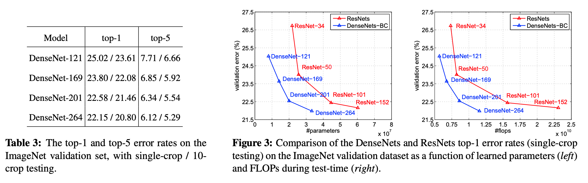
return x6. Experiment & Results
위와 같은 구조로 실험을 해 보았더니..! 더 적은 param 을 가지고도, 더 좋은 성능을 낼 수 있었습니다.
7. 마무리
마지막으로 팁을 드리자면 사실 코드 두줄만 사용하면 densenet 을 뿅 하고 사용할 수 있습니다. (다 알고 계시겠지만 ㅎㅎ)
from torchvision.models import densenet121

model = densenet121()
리뷰를 통해서는 아이디어와 구조에 대한 이해를 얻으셨으면 좋겠습니다.
질문이나 수정할 부분은 언제든지 환영합니다.
감사합니다 뿅:)
torchvision 모델을 활용해서 코드를 짜 보았습니다. :) 참고 부탁드립니다.
github.com/csm-kr/densenet_pytorch/blob/master/densenet2.py
csm-kr/densenet_pytorch
Contribute to csm-kr/densenet_pytorch development by creating an account on GitHub.
github.com
'Network' 카테고리의 다른 글
| [DNN] VGG구현을 위한 리뷰(ICLR 2015) (0) | 2022.07.27 |
|---|---|
| [DNN] ViT 구조 (0) | 2022.06.08 |
| [DNN] Alexnet 리뷰 및 구현 (NIPS 2012) (0) | 2021.09.24 |
| [DNN] U-net 구조와 code 구현 (MICCAI2015) (4) | 2021.05.02 |
| ILSVRC(Imagenet classification)validation set torchvision 으로 성능평가하기 (12) | 2021.03.01 |


댓글