
Introduction
안녕하세요 pulluper입니다. 👏
이번 포스팅에서는 NLP에서 강력한 성능으로 기준이 된 Transformer (Self-Attention)을 vision task에 적용하여 sota(state-of-the-art)의 성능을 달성한 ICLR2021에 발표된 vision transformer에 대한 리뷰 및 구현을 해보겠습니다.
vision에 주로 사용되는 convolution 없이 transformer 만으로 당시 최고의 성능을 달성하였습니다.
약 2년이 지난(2022년 9월 기준) 시기에도 88.55%의 성능으로 26위를 하였고 상위권의 모델들은 대부분 self-attention을 많이 사용했습니다.
이 포스팅의 목표는 ViT의 이해를 통한 간단한 구현입니다.
자 그럼 시작해보겠습니다. 👏👏👏
https://paperswithcode.com/sota/image-classification-on-imagenet
Papers with Code - ImageNet Benchmark (Image Classification)
The current state-of-the-art on ImageNet is CoCa (finetuned). See a full comparison of 707 papers with code.
paperswithcode.com

Inductive bias
Transformer 논문을 보다보면 inductive bias라는 용어를 자주 보실수 있습니다. 위키피디아에서의 inductive bias 의 설명을 보면 다음과 같습니다.
"a learning algorithm is the set of assumptions that the learner uses to predict outputs of given inputs that it has not encountered" - "보지못한 input 에 대한 예측을 하기위해 사용하는 가정의 집합".
학습되는 가정 이라고 생각하는것은 어떨까요? ViT 에서는 다음같은 문장이 있습니다.
"We note that Vision Transformer has much less image-specific inductive bias than CNNs."
ViT가 학습하는데 있어서 input sequence들이 이미지라는 가정이 부족하다는 뜻입니다.
Vision Transformer
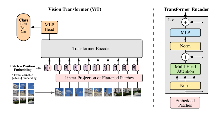
ViT는 또한 NLP 에서 사용한 original Transformer (Vaswani et al., 2017) 최대한 가깝게 만들려고 하였습니다.
기존 논문의 encoder 만을 사용을 하였고 이를 classification 에 잘 적용을 하였습니다.
다음 수식이 ViT의 흐름을 잘 표현해 줍니다. 아래의 각 수식의 (1), (2), (3)을 Embedding, MSA, MLP 부분으로 생각할 수 있습니다.

1. Embedding of ViT
이부분은 이미지를 token화 시키는 부분입니다.
예를들어 다음과 같은 닭이 있을 때, 이것을 token화하는 부분을 알아보겠습니다.
patch 의 크기(P)는 4x4 이고, 이미지의 크기는 32x32 라 했을 때, 8x8=64개의 patch의 갯수가 나옵니다.
각 patch 가 $x_p^1, ...,x_p^N$ 이고 여기에 곱해지는 E(embedding matrix) 는 3차원을 D차원으로 보내주는 trainable linear projection 입니다.
이것은 stride와 kernel size 가 같은 convolution 연산으로 구현 할 수 있습니다.


그리고 $x_{class}$ 는 BERT논문에서 사용되었던 [class] token 입니다.
이는 learnable token으로 nlp 의 classification 을 할 때 sequence전체의 의미를 함축하도록 의도된 learnable parameter 이고, $E_{pos}$는 position embeddings로써, 각 patch의 위치에 더해지는 learnable(sinusoid) parametes입니다.
class token 을 더하기 전의 token의 개수 $N = \frac{H}{P} \times \frac{W}{P} = \frac{H \times W}{P^2}$ 입니다.

Embedding 후 token의 갯수는 N+1 입니다.
여기까지 embedding 부분을 pytorch 코드로 나타내면 다음과 같습니다.
import torch
import torch.nn as nn
from timm.models.layers import trunc_normal_


class EmbeddingLayer(nn.Module):
    def __init__(self, in_chans, embed_dim, img_size, patch_size):
        super().__init__()
        self.num_tokens = (img_size // patch_size) ** 2
        self.embed_dim = embed_dim
        self.project = nn.Conv2d(in_chans, embed_dim, kernel_size=patch_size, stride=patch_size)

        self.cls_token = nn.Parameter(torch.zeros(1, 1, embed_dim))
        self.num_tokens += 1
        self.pos_embed = nn.Parameter(torch.zeros(1, self.num_tokens, self.embed_dim))

        # init cls token and pos_embed -> refer timm vision transformer
        # https://github.com/rwightman/pytorch-image-models/blob/master/timm/models/vision_transformer.py#L391
        nn.init.normal_(self.cls_token, std=1e-6)
        trunc_normal_(self.pos_embed, std=.02)

    def forward(self, x):
        B, C, H, W = x.shape
        embedding = self.project(x)
        z = embedding.view(B, self.embed_dim, -1).permute(0, 2, 1)  # BCHW -> BNC

        # concat cls token
        cls_tokens = self.cls_token.expand(B, -1, -1)
        z = torch.cat([cls_tokens, z], dim=1)

        # add position embedding
        z = z + self.pos_embed
        return z


if __name__ == '__main__':
    img = torch.randn([2, 3, 32, 32])
    embedding = EmbeddingLayer(in_chans=3, embed_dim=192, img_size=32, patch_size=4)
    z = embedding(img)
    print(z.size())
Results: torch.Size([2, 65, 192])
2. MSA(multi-head self-attention)
이번에는 MSA(multi-head self-attetnion) 부분입니다.
위의 과정을 통해서 우리는 [B, N + 1, D] 의 token를 얻을 수 있습니다.
이부분은 milti-head부분과 self attention의 부분으로 설명해 보겠습니다.
multi-head 의 개념의 핵심은 D(e.g.192)의 차원의 token을 head의 갯수로 나누어 head수 만큼 한 이미지(token)에 대하여 여러 관점을 볼 수 있다는 점 입니다.
이는 convolution 의 channel 처럼 생각 할 수 있습니다. 다음 그림은 convit에서 여러 head간 attention map을 시각화 한 것입니다.

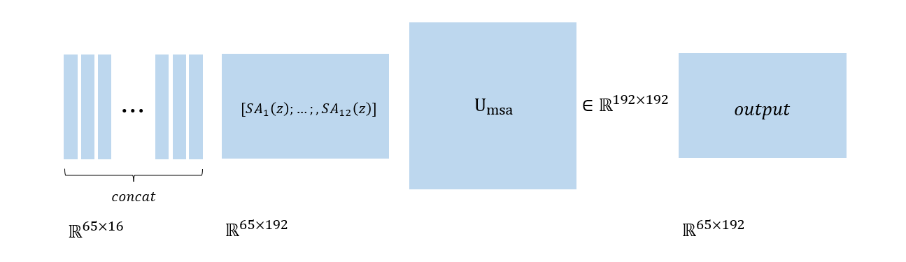
예를들어 N+1 = 65, dim=192, head=12이면 head의 수만큼 token을 다음과 같이 나눌 수 있습니다.
Multi-head로 각각 나눠진 token들 ($\in \mathbb{R}^{64 \times 16}$) 은 각각 self-attention 을 통과해서 $SA_k(z)$ (k는 head의 index)로 연산됩니다.

이후 Self Attention을 통과한 각 head의 값들은 concat이 되어서 마지막 linear projection($U_{msa}$)를 통해서 msa의 값이 나오게 됩니다.
이번에는 Self-Attention 부분입니다.
이를 좀더 자세히 보자면, input token에 대하여 $Q_w, K_w, V_w$ 의 projection matrix를 곱해서 Q, K, V 를 만들고 Q와 K를 dot product 한 부분에 K의 dimension으로 나누는 sclaed dot product 를 진행합니다.
이후 이 값에 softmax를 취하고 V를 곱해줍니다.
여기서 주목할 부분은 softmax의 dim이 -1입니다. 즉, 가로줄의 방향으로 softmax가 진행이 되고, V를 곱해줄 때, 각 token에 대한 normalization된 score를 곱해줄 수 있게 됩니다.
그렇다면, 연산 이후의 값은 softmax(QK/d_k)를 통해서 확률적 score부분이 normalized된 attention 정보를 주게되고, 그 종합적인 정보를 V에 곱하면서 전체 token의 중요성을 고려한 token 값으로 학습되게 하는것 입니다.

이를 실제 구현하는 코드는 다음과 같습니다.
여기서 multi-head를 위해서 각 head로 나눠진 input의 $Q_w, K_w, V_w$ 를 따로 생성하지 않고 한번에 생성을 해서 reshape 와 permute(transpose)를 통해서 병렬적으로 연산하도록 구현됩니다.
import torch.nn as nn

class MSA(nn.Module):
    def __init__(self, dim=192, num_heads=12, qkv_bias=False, attn_drop=0., proj_drop=0.):
        super().__init__()
        assert dim % num_heads == 0, 'dim should be divisible by num_heads'
        self.num_heads = num_heads
        head_dim = dim // num_heads
        self.scale = head_dim ** -0.5

        self.qkv = nn.Linear(dim, dim * 3, bias=qkv_bias)
        self.attn_drop = nn.Dropout(attn_drop)
        self.proj = nn.Linear(dim, dim)
        self.proj_drop = nn.Dropout(proj_drop)

    def forward(self, x):
        B, N, C = x.shape
        qkv = self.qkv(x).reshape(B, N, 3, self.num_heads, C // self.num_heads).permute(2, 0, 3, 1, 4)
        q, k, v = qkv.unbind(0)

        attn = (q @ k.transpose(-2, -1)) * self.scale

        attn = attn.softmax(dim=-1)
        attn = self.attn_drop(attn)

        x = (attn @ v).transpose(1, 2).reshape(B, N, C)
        x = self.proj(x)
        x = self.proj_drop(x)
        return x

if __name__ == '__main__':
    img = torch.randn([2, 3, 32, 32])
    embedding = EmbeddingLayer(in_chans=3, embed_dim=192, img_size=32, patch_size=4)
    z = embedding(img)
    msa = MSA()
    print(msa(z).size())
Results: torch.Size([2, 65, 192])
3. MLP & Block(Transformer Encoder)
마지막으로 MLP부분입니다.
Transformer Encoder 부분은 MSA와 MLP로 이루어져 있고, 이것이 L층 쌓여져 있습니다.
여기서는 Normalization 과 Residual connection 이 사용되었습니다.
먼저 MLP를 보면, input feature 에서 hidden feature로 가는 fc와 (activation 포함) 다시 hidden feature에서 input feature로 가는 fc로 이루어져 있습니다.
원래 논문의 이미지넷에서의 hidden feature의 dim은 4배 늘어서 768 -> 3072로 연산을 합니다.
이 코드에서는 cifar dataset을 사용하기에 hidden feature의 dim은 2배를 늘려서 (192 * 2 ) = 384를 사용합니다.
class MLP(nn.Module):
    def __init__(self, in_features, hidden_features, act_layer=nn.GELU, bias=True, drop=0.):
        super().__init__()
        out_features = in_features

        self.fc1 = nn.Linear(in_features, hidden_features, bias=bias)
        self.act = act_layer()
        self.drop1 = nn.Dropout(drop)
        self.fc2 = nn.Linear(hidden_features, out_features, bias=bias)
        self.drop2 = nn.Dropout(drop)

    def forward(self, x):
        x = self.fc1(x)
        x = self.act(x)
        x = self.drop1(x)
        x = self.fc2(x)
        x = self.drop2(x)
        return x
이후 Transformer Encoder 구현에서는 수식 (2), (3), (4) 를 모두 아우르는 Block이라는 class를 만들어서 Encoder를 구성합니다.
여기서 Encoder는 Fig9. 의 오른쪽과 같이 norm과 residual 구조가 포함됩니다.
class Block(nn.Module):

    def __init__(self, dim, num_heads, mlp_ratio=4., qkv_bias=False,
                 drop=0., attn_drop=0., act_layer=nn.GELU, norm_layer=nn.LayerNorm,
                 ):
        super().__init__()
        self.norm1 = norm_layer(dim)
        self.norm2 = norm_layer(dim)
        self.attn = MSA(dim, num_heads=num_heads, qkv_bias=qkv_bias, attn_drop=attn_drop, proj_drop=drop)
        self.mlp = MLP(in_features=dim, hidden_features=int(dim * mlp_ratio), act_layer=act_layer, drop=drop)

    def forward(self, x):
        x = x + self.attn(self.norm1(x))
        x = x + self.mlp(self.norm2(x))
        return x
마지막으로 ViT class를 여태까지의 모듈들로 구현하면 다음과 같습니다.
depth는 layer의 갯수입니다.
class ViT(nn.Module):
    def __init__(self, img_size=32, patch_size=4, in_chans=3, num_classes=10, embed_dim=192, depth=12,
                 num_heads=12, mlp_ratio=2., qkv_bias=False, drop_rate=0., attn_drop_rate=0.):
        super().__init__()
        self.num_classes = num_classes
        self.num_features = self.embed_dim = embed_dim  # num_features for consistency with other models
        norm_layer = nn.LayerNorm
        act_layer = nn.GELU

        self.patch_embed = EmbeddingLayer(in_chans, embed_dim, img_size, patch_size)
        self.blocks = nn.Sequential(*[
            Block(
                dim=embed_dim, num_heads=num_heads, mlp_ratio=mlp_ratio, qkv_bias=qkv_bias, drop=drop_rate,
                attn_drop=attn_drop_rate, norm_layer=norm_layer, act_layer=act_layer)
            for i in range(depth)])

        # final norm
        self.norm = norm_layer(embed_dim)

        # Classifier head(s)
        self.head = nn.Linear(self.num_features, num_classes) if num_classes > 0 else nn.Identity()

    def forward(self, x):
        x = self.patch_embed(x)
        x = self.blocks(x)
        x = self.norm(x)
        x = self.head(x)[:, 0]
        return x
코드는 많은 부분을 https://github.com/rwightman/pytorch-image-models/blob/master/timm/models/vision_transformer.py 을 사용했습니다. (timm.models.vision_transformer)
이제 구현한 ViT을 통해서 cifar10을 학습시켜보는 예제 코드를 마지막으로 포스팅을 마무리하겠습니다.
학습환경은 다음과 같습니다.
- epoch : 50
- batch_size : 128
- init learning rate : 0.001
- optimizer : Adam(weight_decay : 5e-5)
- model : ViT(img_size=32, patch_size=4, in_chans=3, num_classes=10, embed_dim=192, depth=12,
num_heads=12, mlp_ratio=2., qkv_bias=False, drop_rate=0., attn_drop_rate=0.)
c.f.) model params는 Vision Transformer for Small-Size Datasets (https://arxiv.org/pdf/2112.13492.pdf)를 따랐습니다.
- loss : cross entropy
- dataset : cifar10 (torchvision.data)
- data augmentation : random crop, horizontal random flip
import os
import time
import torch
import visdom
import argparse
import torch.nn as nn
import torchvision.transforms as tfs
from torch.utils.data import DataLoader
from timm.models.layers import trunc_normal_
from torchvision.datasets.cifar import CIFAR10


class EmbeddingLayer(nn.Module):
    def __init__(self, in_chans, embed_dim, img_size, patch_size):
        super().__init__()
        self.num_tokens = (img_size // patch_size) ** 2
        self.embed_dim = embed_dim
        self.project = nn.Conv2d(in_chans, embed_dim, kernel_size=patch_size, stride=patch_size)

        self.cls_token = nn.Parameter(torch.zeros(1, 1, embed_dim))
        self.num_tokens += 1
        self.pos_embed = nn.Parameter(torch.zeros(1, self.num_tokens, self.embed_dim))

        # init cls token and pos_embed -> refer timm vision transformer
        # https://github.com/rwightman/pytorch-image-models/blob/master/timm/models/vision_transformer.py#L391
        nn.init.normal_(self.cls_token, std=1e-6)
        trunc_normal_(self.pos_embed, std=.02)

    def forward(self, x):
        B, C, H, W = x.shape
        embedding = self.project(x)
        z = embedding.view(B, self.embed_dim, -1).permute(0, 2, 1)  # BCHW -> BNC

        # concat cls token
        cls_tokens = self.cls_token.expand(B, -1, -1)
        z = torch.cat([cls_tokens, z], dim=1)

        # add position embedding
        z = z + self.pos_embed
        return z


class MSA(nn.Module):
    def __init__(self, dim=192, num_heads=12, qkv_bias=False, attn_drop=0., proj_drop=0.):
        super().__init__()
        assert dim % num_heads == 0, 'dim should be divisible by num_heads'
        self.num_heads = num_heads
        head_dim = dim // num_heads
        self.scale = head_dim ** -0.5

        self.qkv = nn.Linear(dim, dim * 3, bias=qkv_bias)
        self.attn_drop = nn.Dropout(attn_drop)
        self.proj = nn.Linear(dim, dim)
        self.proj_drop = nn.Dropout(proj_drop)

    def forward(self, x):
        B, N, C = x.shape
        qkv = self.qkv(x).reshape(B, N, 3, self.num_heads, C // self.num_heads).permute(2, 0, 3, 1, 4)
        q, k, v = qkv.unbind(0)

        attn = (q @ k.transpose(-2, -1)) * self.scale

        attn = attn.softmax(dim=-1)
        attn = self.attn_drop(attn)

        x = (attn @ v).transpose(1, 2).reshape(B, N, C)
        x = self.proj(x)
        x = self.proj_drop(x)
        return x


class MLP(nn.Module):
    def __init__(self, in_features, hidden_features, act_layer=nn.GELU, bias=True, drop=0.):
        super().__init__()
        out_features = in_features

        self.fc1 = nn.Linear(in_features, hidden_features, bias=bias)
        self.act = act_layer()
        self.drop1 = nn.Dropout(drop)
        self.fc2 = nn.Linear(hidden_features, out_features, bias=bias)
        self.drop2 = nn.Dropout(drop)

    def forward(self, x):
        x = self.fc1(x)
        x = self.act(x)
        x = self.drop1(x)
        x = self.fc2(x)
        x = self.drop2(x)
        return x


class Block(nn.Module):

    def __init__(self, dim, num_heads, mlp_ratio=4., qkv_bias=False,
                 drop=0., attn_drop=0., act_layer=nn.GELU, norm_layer=nn.LayerNorm,
                 ):
        super().__init__()
        self.norm1 = norm_layer(dim)
        self.norm2 = norm_layer(dim)
        self.attn = MSA(dim, num_heads=num_heads, qkv_bias=qkv_bias, attn_drop=attn_drop, proj_drop=drop)
        self.mlp = MLP(in_features=dim, hidden_features=int(dim * mlp_ratio), act_layer=act_layer, drop=drop)

    def forward(self, x):
        x = x + self.attn(self.norm1(x))
        x = x + self.mlp(self.norm2(x))
        return x


class ViT(nn.Module):
    def __init__(self, img_size=32, patch_size=4, in_chans=3, num_classes=10, embed_dim=192, depth=12,
                 num_heads=12, mlp_ratio=2., qkv_bias=False, drop_rate=0., attn_drop_rate=0.):
        super().__init__()
        self.num_classes = num_classes
        self.num_features = self.embed_dim = embed_dim  # num_features for consistency with other models
        norm_layer = nn.LayerNorm
        act_layer = nn.GELU

        self.patch_embed = EmbeddingLayer(in_chans, embed_dim, img_size, patch_size)
        self.blocks = nn.Sequential(*[
            Block(
                dim=embed_dim, num_heads=num_heads, mlp_ratio=mlp_ratio, qkv_bias=qkv_bias, drop=drop_rate,
                attn_drop=attn_drop_rate, norm_layer=norm_layer, act_layer=act_layer)
            for i in range(depth)])

        # final norm
        self.norm = norm_layer(embed_dim)

        # Classifier head(s)
        self.head = nn.Linear(self.num_features, num_classes) if num_classes > 0 else nn.Identity()

    def forward(self, x):
        x = self.patch_embed(x)
        x = self.blocks(x)
        x = self.norm(x)
        x = self.head(x)[:, 0]
        return x

def main():
    # 1. ** argparser **
    parer = argparse.ArgumentParser()
    parer.add_argument('--epoch', type=int, default=50)
    parer.add_argument('--batch_size', type=int, default=128)
    parer.add_argument('--lr', type=float, default=0.001)
    parer.add_argument('--step_size', type=int, default=100)
    parer.add_argument('--root', type=str, default='./CIFAR10')
    parer.add_argument('--log_dir', type=str, default='./log')
    parer.add_argument('--name', type=str, default='vit_cifar10')
    parer.add_argument('--rank', type=int, default=0)
    ops = parer.parse_args()

    # 2. ** device **
    device = torch.device('cuda:{}'.format(0) if torch.cuda.is_available() else 'cpu')

    # 3. ** visdom **
    vis = visdom.Visdom(port=8097)

    # 4. ** dataset / dataloader **
    transform_cifar = tfs.Compose([
        tfs.RandomCrop(32, padding=4),
        tfs.RandomHorizontalFlip(),
        tfs.ToTensor(),
        tfs.Normalize(mean=(0.4914, 0.4822, 0.4465),
                      std=(0.2023, 0.1994, 0.2010)),
    ])

    test_transform_cifar = tfs.Compose([tfs.ToTensor(),
                                        tfs.Normalize(mean=(0.4914, 0.4822, 0.4465),
                                                      std=(0.2023, 0.1994, 0.2010)),
                                        ])
    train_set = CIFAR10(root=ops.root,
                        train=True,
                        download=True,
                        transform=transform_cifar)

    test_set = CIFAR10(root=ops.root,
                       train=False,
                       download=True,
                       transform=test_transform_cifar)

    train_loader = DataLoader(dataset=train_set,
                              shuffle=True,
                              batch_size=ops.batch_size)

    test_loader = DataLoader(dataset=test_set,
                             shuffle=False,
                             batch_size=ops.batch_size)

    # 5. ** model **
    model = ViT().to(device)

    # 6. ** criterion **
    criterion = nn.CrossEntropyLoss()

    # 7. ** optimizer **
    optimizer = torch.optim.Adam(model.parameters(),
                                 lr=ops.lr,
                                 weight_decay=5e-5)

    # 8. ** scheduler **
    scheduler = torch.optim.lr_scheduler.CosineAnnealingLR(optimizer, T_max=ops.epoch, eta_min=1e-5)

    # 9. ** logger **
    os.makedirs(ops.log_dir, exist_ok=True)

    # 10. ** training **
    print("training...")
    for epoch in range(ops.epoch):

        model.train()
        tic = time.time()
        for idx, (img, target) in enumerate(train_loader):
            img = img.to(device)  # [N, 3, 32, 32]
            target = target.to(device)  # [N]
            # output, attn_mask = model(img, True)  # [N, 10]
            output = model(img)  # [N, 10]
            loss = criterion(output, target)

            optimizer.zero_grad()
            loss.backward()
            optimizer.step()

            for param_group in optimizer.param_groups:
                lr = param_group['lr']

            if idx % ops.step_size == 0:
                vis.line(X=torch.ones((1, 1)) * idx + epoch * len(train_loader),
                         Y=torch.Tensor([loss]).unsqueeze(0),
                         update='append',
                         win='training_loss',
                         opts=dict(x_label='step',
                                   y_label='loss',
                                   title='loss',
                                   legend=['total_loss']))

                print('Epoch : {}\t'
                      'step : [{}/{}]\t'
                      'loss : {}\t'
                      'lr   : {}\t'
                      'time   {}\t'
                      .format(epoch,
                              idx, len(train_loader),
                              loss,
                              lr,
                              time.time() - tic))

        # save
        save_path = os.path.join(ops.log_dir, ops.name, 'saves')
        os.makedirs(save_path, exist_ok=True)

        checkpoint = {'epoch': epoch,
                      'model_state_dict': model.state_dict(),
                      'optimizer_state_dict': optimizer.state_dict(),
                      'scheduler_state_dict': scheduler.state_dict()}

        torch.save(checkpoint, os.path.join(save_path, ops.name + '.{}.pth.tar'.format(epoch)))

        # 10. ** test **
        print('Validation of epoch [{}]'.format(epoch))
        model.eval()
        correct = 0
        val_avg_loss = 0
        total = 0
        with torch.no_grad():

            for idx, (img, target) in enumerate(test_loader):
                model.eval()
                img = img.to(device)  # [N, 3, 32, 32]
                target = target.to(device)  # [N]
                output = model(img)  # [N, 10]
                loss = criterion(output, target)

                output = torch.softmax(output, dim=1)
                # first eval
                pred, idx_ = output.max(-1)
                correct += torch.eq(target, idx_).sum().item()
                total += target.size(0)
                val_avg_loss += loss.item()

        print('Epoch {} test : '.format(epoch))
        accuracy = correct / total
        print("accuracy : {:.4f}%".format(accuracy * 100.))

        val_avg_loss = val_avg_loss / len(test_loader)
        print("avg_loss : {:.4f}".format(val_avg_loss))

        if vis is not None:
            vis.line(X=torch.ones((1, 2)) * epoch,
                     Y=torch.Tensor([accuracy, val_avg_loss]).unsqueeze(0),
                     update='append',
                     win='test_loss',
                     opts=dict(x_label='epoch',
                               y_label='test_',
                               title='test_loss',
                               legend=['accuracy', 'avg_loss']))
        scheduler.step()


if __name__ == '__main__':
    main()
결과는 다음과 같습니다.
- training/test loss plot and accuracy


50 epoch 을 모두 돌렸을 때의 성능은 77~78%의 성능이 나옴을 알 수 있었습니다.
이번 포스팅에서는 ViT의 논문리뷰와 구현을 알아보았습니다.
다음에는 구체적인 DATA augmentation과 학습 방법에 대하여 알아보겠습니다. 감사합니다. 👍👍👍
'Network' 카테고리의 다른 글
| [DNN] multi-head cross attention vs multi-head self attention 비교 (0) | 2023.02.02 |
|---|---|
| performer 구현 (0) | 2022.12.12 |
| [DNN] Resnet 리뷰/구조 (CVPR2016) (2) | 2022.08.29 |
| [DNN] VGG구현을 위한 리뷰(ICLR 2015) (0) | 2022.07.27 |
| [DNN] ViT 구조 (1) | 2022.06.08 |


댓글